Student contact network at school: Spread of the virus
By Byoung-gyu Gong
Pandemic and School Reopening Issue
With an outbreak of the COVID-19 pandemic, there is increasing attention to the school closer issue. Many countries implemented a strict lock-down to slow down the spread of the virus, but this came at the expense of losing our children’s learning opportunity. Despite that, the reopening school can be very costly as children can transmit the virus to their families and communities. Now that there is significant uncertainty on the impact of school reopening, we see that many countries are still under discussion on this issue. Disappointingly, we do not know much about how the school affects the children’s virus infection.
Purpose of the Analysis
Given this situation, in this post, I will analyze children’s physical contact network at school to see how much contact happens among children. The contact network indicators at school can be a basic knowledge we can reorganize our school space, time, and activity to adjust to the post-pandemic world.
Data Source
For the network analysis, I prepared two data sets from the study of Gemnetto, Barrat, & Cattuto (2014) titled Mitigation of infectious disease at school: Targeted class closure vs school closure, which studied the infection network at the primary school. You can also find the data of this study from Sociopatterns. It is the open-source network data platform readily available for any studies and researches. The students’ contact network data provides a fundamental sense to design and implement a plan for contact tracing and social distance at each school level.
The authors collected this contact network data using a wearable device that records contact whenever students get closer over a certain threshold. The data was collected from an elementary school in France.
Analysis
For the analysis, I will use igraph package in R program. Using this package, I will calculate centrality scores to detect the central node in the school network and network structure indicators, such as network density and homophily score. Also, I will visualize the network to show you the birds-eye view of the school network.
Data pre-processing
First, install the required packages and open the library.
install.packages(c("igraph","readr","tidyr","RColorBrewer"))Then, you can download the data file directly from my github repository through the following code. (If there is an error message, you should try it multiple times until you can get access to it.)
#1. Read data from the Github repository csv files
urlfile1="https://raw.githubusercontent.com/Arizonagong/vCIES2020_Network-Analysis/master/igraph/primaryschool.csv"
urlfile2="https://raw.githubusercontent.com/Arizonagong/vCIES2020_Network-Analysis/master/igraph/metadata_primaryschool.csv"
D<-read_csv(url(urlfile1))
##
## ── Column specification ────────────────────────────────────────────
## cols(
## Source = col_double(),
## Target = col_double()
## )D_meta<-read_csv(url(urlfile2))##
## ── Column specification ────────────────────────────────────────────
## cols(
## ID = col_double(),
## Class = col_character(),
## Gender = col_character()
## )Now, let’s look into the data set. The first dataset names as “D” is an edge list indicating contact between the students. It is represented like 1234-4424, which means one contact between the student 1234 and 4424.
head(D, 5)## # A tibble: 5 x 2
## Source Target
## <dbl> <dbl>
## 1 1558 1567
## 2 1560 1570
## 3 1567 1574
## 4 1632 1818
## 5 1632 1866The data set “D_meta” includes node information with students ID, class, and gender information.
head(D_meta, 5)## # A tibble: 5 x 3
## ID Class Gender
## <dbl> <chr> <chr>
## 1 1426 5B M
## 2 1427 5B F
## 3 1428 5B M
## 4 1429 5B F
## 5 1430 5B MThen, I just created “frequency” column in the edgelist, “D” to give an edge attribute for each edges with their contact frequency, and deleted all edges having 0 contact.
#2. Manage dataset
B<-as.data.frame(table(D)) # Create an edge weight column named "Freq"
B1<-subset(B,Freq>0) # Delete all the edges having weight equal to 0
head(B1, 5)
## Source Target Freq
## 1 1426 1427 27
## 240 1426 1428 45
## 241 1427 1428 4
## 479 1426 1429 75
## 480 1427 1429 100Then, we can now create an igraph object. igraph object is different from the data frame and requires totally different grammar from the code handling general data frame. igraph is specially designed to handle large-sized complex network data with high speed. The igraph object, “Stucont” includes edgelist, nodelist, and their attributes.
#3. Create an igraph object from the dataframes
Stucont<-graph_from_data_frame(B1, directed = FALSE, vertices = D_meta)
E(Stucont)$weight<-E(Stucont)$Freq # Assigning edge attribute to each edge
Stucont
## IGRAPH 31f002e UNW- 242 8317 --
## + attr: name (v/c), Class (v/c), Gender (v/c), Freq (e/n), weight (e/n)
## + edges from 31f002e (vertex names):
## [1] 1426--1427 1426--1428 1427--1428 1426--1429 1427--1429 1428--1429
## [7] 1426--1430 1427--1430 1428--1430 1429--1430 1426--1431 1427--1431
## [13] 1428--1431 1429--1431 1430--1431 1426--1434 1427--1434 1428--1434
## [19] 1429--1434 1430--1434 1431--1434 1426--1435 1427--1435 1428--1435
## [25] 1429--1435 1430--1435 1431--1435 1434--1435 1426--1437 1427--1437
## [31] 1428--1437 1429--1437 1430--1437 1431--1437 1434--1437 1435--1437
## [37] 1426--1439 1427--1439 1428--1439 1429--1439 1430--1439 1431--1439
## [43] 1434--1439 1435--1439 1437--1439 1426--1441 1427--1441 1428--1441
## + ... omitted several edgesExploring basic network features
gsize shows us the number of edges, and gorder shows the number of nodes
gsize(Stucont)## [1] 8317gorder(Stucont)## [1] 242V means the vertex (node), so with this function you can see the nodelist.
#2. Nodelist
V(Stucont)
## + 242/242 vertices, named, from 31f002e:
## [1] 1426 1427 1428 1429 1430 1431 1434 1435 1437 1439 1441 1443 1451 1452 1453
## [16] 1457 1458 1459 1461 1465 1468 1471 1475 1477 1479 1480 1482 1483 1486 1489
## [31] 1493 1495 1498 1500 1501 1502 1503 1504 1511 1516 1519 1520 1521 1522 1524
## [46] 1525 1528 1532 1533 1538 1539 1545 1546 1548 1549 1551 1552 1555 1558 1560
## [61] 1562 1563 1564 1567 1570 1572 1574 1578 1579 1580 1585 1592 1594 1601 1603
## [76] 1604 1606 1609 1613 1616 1617 1618 1625 1628 1630 1632 1637 1641 1643 1647
## [91] 1648 1649 1650 1653 1656 1661 1663 1664 1665 1666 1668 1670 1673 1674 1675
## [106] 1680 1681 1682 1684 1685 1687 1688 1695 1696 1697 1698 1700 1702 1704 1705
## [121] 1706 1707 1708 1709 1710 1711 1712 1713 1714 1715 1718 1719 1720 1722 1723
## [136] 1727 1730 1731 1732 1735 1737 1738 1739 1741 1743 1744 1745 1746 1748 1749
## + ... omitted several verticesE means the edge.
#3. Edgelist
E(Stucont)
## + 8317/8317 edges from 31f002e (vertex names):
## [1] 1426--1427 1426--1428 1427--1428 1426--1429 1427--1429 1428--1429
## [7] 1426--1430 1427--1430 1428--1430 1429--1430 1426--1431 1427--1431
## [13] 1428--1431 1429--1431 1430--1431 1426--1434 1427--1434 1428--1434
## [19] 1429--1434 1430--1434 1431--1434 1426--1435 1427--1435 1428--1435
## [25] 1429--1435 1430--1435 1431--1435 1434--1435 1426--1437 1427--1437
## [31] 1428--1437 1429--1437 1430--1437 1431--1437 1434--1437 1435--1437
## [37] 1426--1439 1427--1439 1428--1439 1429--1439 1430--1439 1431--1439
## [43] 1434--1439 1435--1439 1437--1439 1426--1441 1427--1441 1428--1441
## [49] 1429--1441 1431--1441 1434--1441 1435--1441 1437--1441 1439--1441
## [55] 1426--1443 1427--1443 1428--1443 1429--1443 1430--1443 1431--1443
## + ... omitted several edgesEach node have attributes such as ID, class, and gender. There are missing values so we will change “unknown” into NA.
#4. Attributes
V(Stucont)$Gender
## [1] "M" "F" "M" "F" "M" "F" "F"
## [8] "M" "F" "M" "M" "F" "F" "M"
## [15] "F" "F" "M" "M" "F" "F" "M"
## [22] "M" "F" "M" "M" "F" "M" "F"
## [29] "M" "F" "F" "M" "M" "M" "F"
## [36] "F" "F" "F" "M" "M" "F" "F"
## [43] "Unknown" "M" "F" "M" "M" "M" "M"
## [50] "F" "F" "M" "F" "M" "M" "M"
## [57] "F" "F" "M" "F" "F" "F" "M"
## [64] "M" "F" "F" "F" "M" "M" "M"
## [71] "M" "M" "M" "F" "F" "F" "F"
## [78] "F" "M" "F" "F" "Unknown" "M" "M"
## [85] "M" "F" "Unknown" "F" "F" "M" "F"
## [92] "M" "Unknown" "Unknown" "M" "F" "F" "M"
## [99] "M" "M" "Unknown" "F" "M" "F" "F"
## [106] "F" "M" "F" "F" "F" "F" "M"
## [113] "F" "F" "M" "M" "F" "F" "M"
## [120] "M" "F" "M" "M" "Unknown" "M" "F"
## [127] "F" "F" "M" "F" "F" "F" "F"
## [134] "F" "M" "F" "Unknown" "M" "M" "M"
## [141] "M" "F" "M" "M" "F" "M" "Unknown"
## [148] "Unknown" "M" "F" "M" "F" "M" "Unknown"
## [155] "F" "M" "F" "M" "M" "M" "F"
## [162] "M" "M" "F" "F" "F" "F" "Unknown"
## [169] "F" "M" "M" "M" "M" "F" "M"
## [176] "F" "M" "F" "F" "M" "M" "Unknown"
## [183] "F" "F" "M" "M" "M" "F" "F"
## [190] "F" "M" "F" "M" "F" "M" "Unknown"
## [197] "F" "M" "F" "M" "M" "M" "M"
## [204] "M" "M" "Unknown" "F" "M" "F" "F"
## [211] "F" "F" "M" "M" "M" "F" "F"
## [218] "M" "M" "M" "M" "M" "F" "M"
## [225] "M" "F" "F" "F" "M" "F" "F"
## [232] "M" "M" "F" "M" "M" "F" "M"
## [239] "F" "M" "F" "F"V(Stucont)$Gender[V(Stucont)$Gender=='Unknown'] <- NAThe adjacency matrix is the most important indication of the network. However, igraph does not store the network data in the adjacency matrix format. Still, you can represent the network in the matrix format as below. We can know that the contact network is a symmetric and undirected network from the adjacency matrix, which means there is no arrow on edges.
#5. Adjacency matrix
Stucont[c(1:10),c(1:10)]
## 10 x 10 sparse Matrix of class "dgCMatrix"## [[ suppressing 10 column names '1426', '1427', '1428' ... ]]##
## 1426 . 27 45 75 19 43 8 12 23 27
## 1427 27 . 4 100 4 63 20 5 44 13
## 1428 45 4 . 9 4 16 2 4 19 14
## 1429 75 100 9 . 9 75 11 5 62 36
## 1430 19 4 4 9 . 15 4 7 4 3
## 1431 43 63 16 75 15 . 43 16 42 41
## 1434 8 20 2 11 4 43 . 3 8 8
## 1435 12 5 4 5 7 16 3 . 6 11
## 1437 23 44 19 62 4 42 8 6 . 29
## 1439 27 13 14 36 3 41 8 11 29 .Measuring centrality
Centrality is the most important indicator of the network. The centrality measure shows which node has the highest contact frequency in the network. To understand more about the centrality measure, please visit my lecture page on the Youtube channel. I will not explain the details of each centrality measure in this post.
I identified the nodes recording the highest score in each of the centrality measures and found that student 1551 shows the highest centrality in the degree and betweenness centrality measure.
#1. Degree centrality
Stucont_deg<-degree(Stucont,mode=c("All"))
V(Stucont)$degree<-Stucont_deg
which.max(Stucont_deg)
## 1551
## 56#2. Eigenvector centrality
Stucont_eig <- evcent(Stucont)$vector
V(Stucont)$Eigen<-Stucont_eig
which.max(Stucont_eig)## 1665
## 99#3. Betweenness centrality
Stucont_bw<-betweenness(Stucont, directed = FALSE)
V(Stucont)$betweenness<-Stucont_bw
which.max(Stucont_bw)## 1551
## 56Measuring network structure
Each network has its unique structural features.
First, network density indicates how much densely the nodes are connected in the network. Also, if you’d like to know more about the network theory, please watch my lecture on Youtube.
Here I compared the network density between the school and the class level. It shows that the school level density is 0.28 while the class level density is 0.98. Thus, there is a considerable density gap between the school and the class.
#1. Network Density
edge_density(Stucont) # Global density
## [1] 0.2852097A1<-induced_subgraph(Stucont, V(Stucont)[Class=="1A"], impl=c("auto")) # Subgraphing into each class
edge_density(A1) # Class level density## [1] 0.9841897We can also calculate the assortativity score, which means mingling together with the nodes having a similar attribute. For instance, we can expect that the same class students or having the same gender may have more frequent contact. The assortativity score of the class is 0.23.
#2. Assortativity
values <- as.numeric(factor(V(Stucont)$Class))
assortativity_nominal(Stucont, types=values)
## [1] 0.2337739But, we do not know how big enough or small to assess the level of assortativity. We can then create a random network, which has the same probability of having an edge between every node and comparing it. The histogram indicates that the school network data is such an abnormal case having a high assortativity score according to the random network’s probability distribution.
#2.1. Calculate the observed assortativity
observed.assortativity <- assortativity_nominal(Stucont, types=values)
results <- vector('list', 1000)
for(i in 1:1000){results[[i]] <- assortativity_nominal(Stucont, sample(values))}
#2.2.  Plot the distribution of assortativity values and add a red vertical line at the original observed value
hist(unlist(results), xlim = c(0,0.4))
abline(v = observed.assortativity,col = "red", lty = 3, lwd=2) 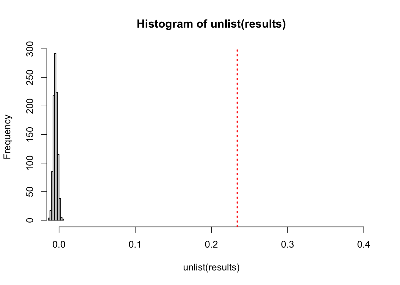
Network Visualization
The final step is the network visualization. The beauty of network analysis is that we can visually confirm the features we indicated by the numbers above. Also, the visual mapping of the network is instrumental in communicating with the audiences with data. Here, I set the size of each node with a value of degree centrality. Each different color indicates different classes.
#1. Plotting a network with the degree centrality
set.seed(1001)
library(RColorBrewer) # This is the color library
pal<-brewer.pal(length(unique(V(Stucont)$Class)), "Set3") # Vertex color assigned per each class number
plot(Stucont,edge.color = 'black',vertex.label.cex =0.5,
     vertex.color=pal[as.numeric(as.factor(vertex_attr(Stucont, "Class")))],
     vertex.size = sqrt(Stucont_deg)/2, edge.width=sqrt(E(Stucont)$weight/800),
     layout = layout.fruchterman.reingold)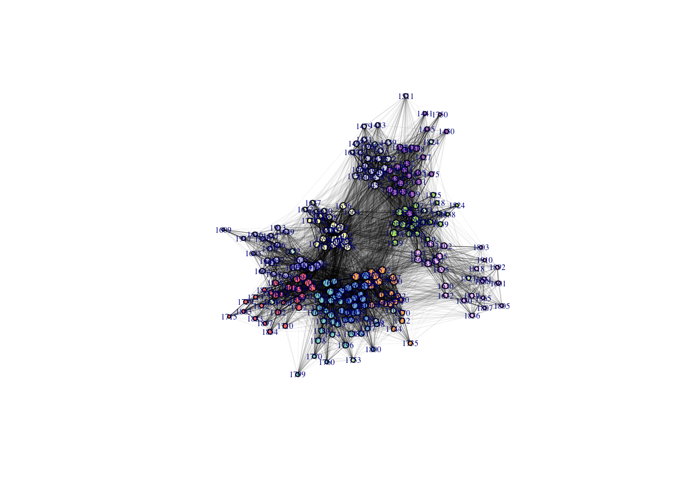
Community Detection
Based on the networking pattern of the node, we can cluster them into several groups. We can intuitively think that the nodes will be clustered based on their affiliation with the classes. However, the result is counter-intuitive. We have ten classes in the school dataset, but the number of detected communities (cluster) is 6, which means that this school is composed of 6 different sub-network groups.
#1. Louvain clustering
lc <- cluster_louvain(Stucont) # Create a cluster based on the Louvain method
communities(lc) # You can check which vertices belongs to which clusters.
## $`1`
## [1] "1426" "1427" "1428" "1429" "1430" "1431" "1434" "1435" "1437" "1439"
## [11] "1441" "1443" "1451" "1452" "1453" "1457" "1458" "1459" "1461" "1465"
## [21] "1468" "1471" "1475" "1477" "1479" "1480" "1482" "1483" "1486" "1489"
## [31] "1493" "1495" "1498" "1501" "1502" "1511" "1516" "1520" "1522" "1563"
## [41] "1578" "1585" "1592" "1637" "1668" "1750" "1751" "1824" "1885"
##
## $`2`
## [1] "1656" "1661" "1663" "1664" "1665" "1666" "1670" "1673" "1674" "1675"
## [11] "1680" "1681" "1682" "1684" "1687" "1688" "1695" "1696" "1697" "1698"
## [21] "1745" "1765" "1779" "1908" "1912" "1920"
##
## $`3`
## [1] "1711" "1752" "1753" "1757" "1759" "1760" "1761" "1764" "1766" "1767"
## [11] "1768" "1770" "1772" "1774" "1775" "1778" "1783" "1787" "1789" "1790"
## [21] "1792" "1796" "1798" "1799"
##
## $`4`
## [1] "1500" "1503" "1504" "1519" "1521" "1524" "1525" "1528" "1532" "1533"
## [11] "1538" "1539" "1545" "1546" "1548" "1549" "1601" "1618" "1630" "1632"
## [21] "1653" "1705" "1730" "1797" "1802" "1803" "1805" "1807" "1815" "1818"
## [31] "1819" "1821" "1831" "1835" "1836" "1837" "1847" "1857" "1865" "1866"
## [41] "1880" "1888" "1892" "1895" "1910"
##
## $`5`
## [1] "1603" "1604" "1606" "1609" "1613" "1616" "1617" "1625" "1628" "1641"
## [11] "1643" "1647" "1648" "1649" "1650" "1702" "1704" "1706" "1708" "1710"
## [21] "1713" "1715" "1718" "1732" "1739" "1743" "1749" "1851" "1852" "1854"
## [31] "1855" "1858" "1861" "1863" "1872" "1877" "1883" "1887" "1889" "1890"
## [41] "1897" "1898" "1902" "1906" "1907" "1911" "1913" "1916" "1917" "1919"
## [51] "1922"
##
## $`6`
## [1] "1551" "1552" "1555" "1558" "1560" "1562" "1564" "1567" "1570" "1572"
## [11] "1574" "1579" "1580" "1594" "1685" "1700" "1707" "1709" "1712" "1714"
## [21] "1719" "1720" "1722" "1723" "1727" "1731" "1735" "1737" "1738" "1741"
## [31] "1744" "1746" "1748" "1763" "1780" "1782" "1795" "1800" "1801" "1809"
## [41] "1820" "1822" "1833" "1838" "1843" "1859" "1909"#2. Plotting the Betweenness Centrality network with the community detection
set.seed(1001) # To duplicate the computer process and create exactly the same network repetitively you should set the seed.
plot(lc, Stucont, edge.color = 'black',vertex.label.cex =0.5,
vertex.color=pal[as.numeric(as.factor(vertex_attr(Stucont, "Class")))],
vertex.size = sqrt(Stucont_bw)/3, edge.width=sqrt(E(Stucont)$weight/800),
layout = layout.fruchterman.reingold)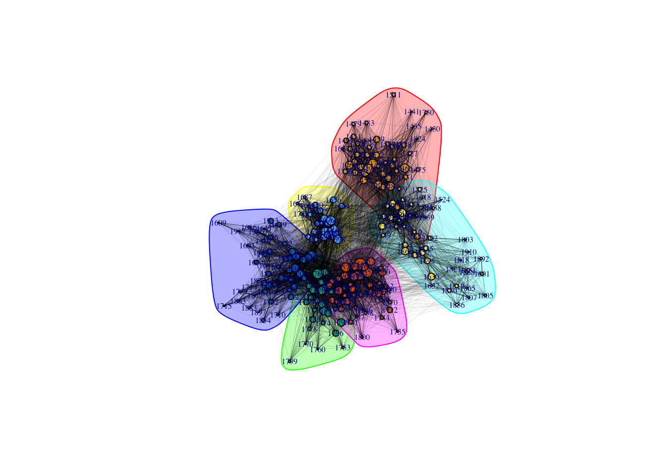
So far, we walked through the whole process of network analysis and visualization. Although this analysis is descriptive, we could learn a lot about the school’s student dynamics only with this small information. Also, it provided information on the latent community structure that was not visible before the analysis.
The students’ physical contact data set is rare because it has a privacy issue to measure the contact information. Thus, this analysis provides us such a precious insight into the students’ physical network in school.