Analyzing Nested Data: Comparing Multiple Approaches
1. What is Nested Data
Not all data is created to be independent. We often find that the real world data does not meet the strict statistical presumption that each observation should be independent and identically distributed, so-called iid. In many cases of social science studies, the observations sampled from a population tend to correlate because they belong to the same group, region, and culture. Sample data having such common and correlative trait is called nested data.
For instance, students in the same school share some traits derived from the school and district features. Students in the same school or district tend to have similar socio-economic status (SES) because students are assigned to the schools based on their residential location. Students in the same school also tend to share the same teachers, school leadership, and school resource. In this account, student samples in the same schools may violate iid principle correlating with each other.
2. Example Data Analysis
It can be costly to ignore the nested data structure. This post will show you a difference between the models considering and not considering the nested data structure.
I used the international students’ data file for this analysis. The students studied in a foreign country through a one-year study abroad program to raise intercultural understanding. I analyzed to what extent the self-efficacy level predicts or explains the level of students’ intercultural understanding.
2.1. Explorative Data Analysis
This is the summary of the data set. It tells us there are four variables. Intercultural_Understanding and Self-Efficacy are the continuous variables while the rest of Major and Year are categorical variables.
# Summary of the data
summary(Studyabroad)
## Intercultural_Understanding Self_Efficacy Major Year
## Min. :1.000 Min. :3.000 Eng :20 18-19:31
## 1st Qu.:3.250 1st Qu.:4.208 Noneng:52 19-20:41
## Median :4.333 Median :5.190
## Mean :4.089 Mean :4.980
## 3rd Qu.:5.000 3rd Qu.:5.762
## Max. :6.000 Max. :6.000
## NA's :2 NA's :1To get a more detailed sense of the data, let’s check the distribution of the data with visualization.
# Scatter plot
SA <- ggscatter(Studyabroad, x = "Self_Efficacy", y = "Intercultural_Understanding",color = "#00AFBB", size = 1, alpha = 0.6, add = "reg.line", add.params = list(color = "blue", fill = "lightgray"),
   conf.int = TRUE,
   cor.coef = TRUE ,rug = TRUE)+
border()
# Marginal density plot of x (top panel) and y (right panel)
xplot <- ggdensity(Studyabroad, "Self_Efficacy", fill = "lightgrey")
yplot <- ggdensity(Studyabroad, "Intercultural_Understanding", fill = "lightgrey")+
rotate()
# Cleaning the plots
SA <- SA + rremove("legend")
yplot <- yplot + clean_theme() + rremove("legend")
xplot <- xplot + clean_theme() + rremove("legend")

library(cowplot)
plot_grid(xplot, NULL, SA, yplot, ncol = 2, align = "hv",
      rel_widths = c(2, 1), rel_heights = c(1, 2))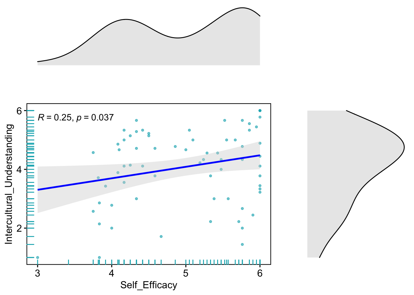
2.2. Simple Linear Regression
The easiest way to analyze this data is simple linear regression. The analysis summary indicates that the students’ self-efficacy is positively associated with the level of intercultural understanding. The coefficient estimate is 0.3914, and the p-value is significant at the 0.05 level.
Lm0<-lm(Intercultural_Understanding ~ Self_Efficacy, data =  Studyabroad)
summary(Lm0)
##
## Call:
## lm(formula = Intercultural_Understanding ~ Self_Efficacy, data = Studyabroad)
##
## Residuals:
## Min 1Q Median 3Q Max
## -2.9404 -0.9175 0.2527 0.9850 1.8409
##
## Coefficients:
## Estimate Std. Error t value Pr(>|t|)
## (Intercept) 2.1298 0.9314 2.287 0.0254 *
## Self_Efficacy 0.3914 0.1841 2.126 0.0372 *
## ---
## Signif. codes: 0 '***' 0.001 '**' 0.01 '*' 0.05 '.' 0.1 ' ' 1
##
## Residual standard error: 1.253 on 67 degrees of freedom
## (3 observations deleted due to missingness)
## Multiple R-squared: 0.06319, Adjusted R-squared: 0.04921
## F-statistic: 4.52 on 1 and 67 DF, p-value: 0.03722.3. Alternative Analytic Methods for the Nested Data
However, the data is stratified with other grouping variables. The data ‘Studyabroad’ has a ‘Major’ variable, indicating that each student belongs to a specific major program. The students’ intercultural understanding explained by self-efficacy may be influenced by their majors.
We can plot the regression line in the above scatter plot, but I will draw two different lines for each group this time. The scatter plot below shows that students in English and non-English majors have very different patterns of association. In general, the students’ intercultural understanding in English majors is related to their self-efficacy level, while the non-English major students showed no relationship between them.
SA<-ggscatter(Studyabroad, x = "Self_Efficacy", y = "Intercultural_Understanding", size = 0.3,
          combine = TRUE, color = "Major", palette = "jco",
          add = "reg.line", conf.int = TRUE) +
  stat_cor(aes(color = Major), method = "spearman")
# Marginal density plot of x (top panel) and y (right panel)
xplot <- ggdensity(Studyabroad, "Self_Efficacy", fill = "Major",
                   palette = "jco")
yplot <- ggdensity(Studyabroad, "Intercultural_Understanding", fill = "Major",palette = "jco")+
rotate()
# Cleaning the plots
SA <- SA + rremove("legend")
yplot <- yplot + clean_theme() + rremove("legend")
xplot <- xplot + clean_theme() + rremove("legend")

library(cowplot)
plot_grid(xplot, NULL, SA, yplot, ncol = 2, align = "hv",
      rel_widths = c(2, 1), rel_heights = c(1, 2))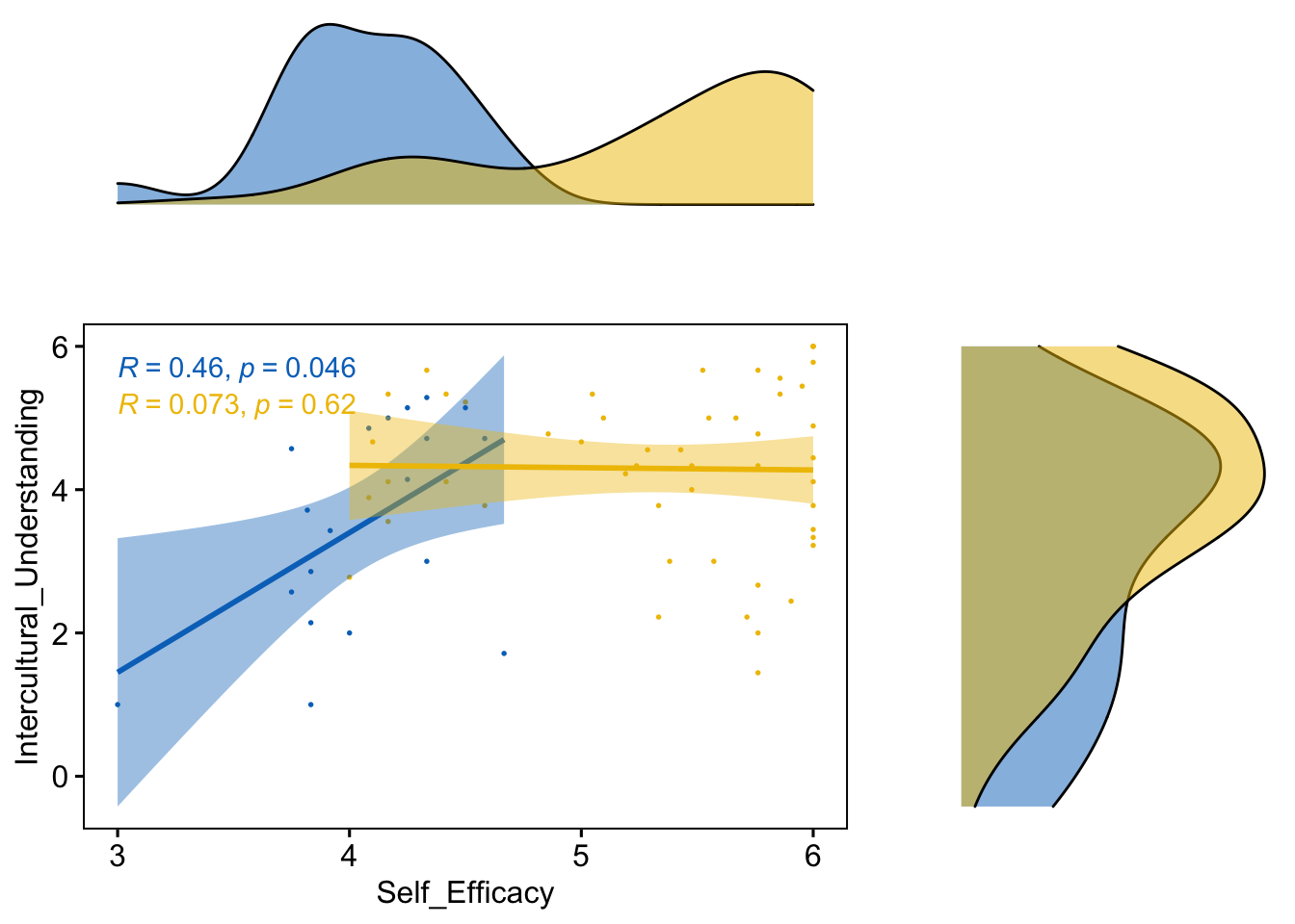
The biggest problem of not considering the nested structure of the data is underestimating each parameter estimation’s standard error. This underestimation is fed into a more frequent rejection of the null hypothesis for the coefficient estimation. We have already seen that the simple linear regression model rejected the null hypothesis above.
2.3.1. Solution1. Complex Linear Regression Model with Grouping Dummy Variables
One of the immediate solutions to handle nested data issue is adding grouping dummy variables in the regression modeling.
The new regression model below included ‘Major,’ one of the grouping variables, in the modeling. Comparing with the previous simple linear regression, the standard error of Self-efficacy’s coefficient increased from 0.1841 to 0.2565. Moreover, the significant test of the coefficient estimation did not reject the null hypothesis.
Lm1<-lm(Intercultural_Understanding ~ Self_Efficacy + Major, data =  Studyabroad)
summary(Lm1)
##
## Call:
## lm(formula = Intercultural_Understanding ~ Self_Efficacy + Major,
## data = Studyabroad)
##
## Residuals:
## Min 1Q Median 3Q Max
## -2.93139 -0.89425 0.05834 1.09501 1.70774
##
## Coefficients:
## Estimate Std. Error t value Pr(>|t|)
## (Intercept) 2.7438 1.0816 2.537 0.0136 *
## Self_Efficacy 0.1925 0.2565 0.750 0.4557
## MajorNoneng 0.5228 0.4706 1.111 0.2706
## ---
## Signif. codes: 0 '***' 0.001 '**' 0.01 '*' 0.05 '.' 0.1 ' ' 1
##
## Residual standard error: 1.251 on 66 degrees of freedom
## (3 observations deleted due to missingness)
## Multiple R-squared: 0.08039, Adjusted R-squared: 0.05253
## F-statistic: 2.885 on 2 and 66 DF, p-value: 0.062932.3.2. Solution2. Hierarchical Linear Modeling (HLM) or Multilevel Modeling
Then, at this time, I will use hierarchical linear modeling analysis with the lme4 package to compare it with the previous simple linear regression model.
First, I will create a null model to calculate the intraclass correlation (ICC). This number indicates the proportion of the outcome variable’s total variation explained by between-group variation. The ICC calculation for this data is about 12%, meaning that the students’ difference in affiliation to majors explains the 12% out of the total variation of the intercultural understanding.
library(lme4)
Lme0<-lmer(Intercultural_Understanding ~ 1+(1|Major), data=Studyabroad)
summary(Lme0)
## Linear mixed model fit by REML ['lmerMod']
## Formula: Intercultural_Understanding ~ 1 + (1 | Major)
## Data: Studyabroad
##
## REML criterion at convergence: 231.6
##
## Scaled residuals:
## Min 1Q Median 3Q Max
## -2.2609 -0.6583 0.1094 0.8609 1.4064
##
## Random effects:
## Groups Name Variance Std.Dev.
## Major (Intercept) 0.2082 0.4563
## Residual 1.5430 1.2422
## Number of obs: 70, groups: Major, 2
##
## Fixed effects:
## Estimate Std. Error t value
## (Intercept) 3.9655 0.3606 10.99# ICC Calculation
library(sjstats)
icc(Lme0)## # Intraclass Correlation Coefficient
##
## Adjusted ICC: 0.119
## Conditional ICC: 0.119Then, I added self-efficacy as a predictor. The summary statistics indicate that the self-efficacy coefficient is not significant due to its increased standard error estimation. This tells us that similar to the regression model with the grouping dummy variables, the multilevel modeling also avoids underestimating the standard error lowering probability to reject the null hypothesis.
library(lmerTest)
Lme1<-lmer(Intercultural_Understanding ~ 1 + Self_Efficacy + (1+Self_Efficacy|Major), data=Studyabroad, na.action = na.exclude)
summary(Lme1)
## Linear mixed model fit by REML. t-tests use Satterthwaite's method [
## lmerModLmerTest]
## Formula:
## Intercultural_Understanding ~ 1 + Self_Efficacy + (1 + Self_Efficacy |
## Major)
## Data: Studyabroad
##
## REML criterion at convergence: 223.9
##
## Scaled residuals:
## Min 1Q Median 3Q Max
## -2.4245 -0.5919 0.1211 0.8689 1.4253
##
## Random effects:
## Groups Name Variance Std.Dev. Corr
## Major (Intercept) 34.365 5.862
## Self_Efficacy 1.717 1.310 -1.00
## Residual 1.422 1.193
## Number of obs: 69, groups: Major, 2
##
## Fixed effects:
## Estimate Std. Error df t value Pr(>|t|)
## (Intercept) 0.2977 4.2955 0.6712 0.069 0.960
## Self_Efficacy 0.8874 0.9615 0.6535 0.923 0.582
##
## Correlation of Fixed Effects:
## (Intr)
## Self_Effccy -0.999
## convergence code: 0
## boundary (singular) fit: see ?isSingular3. Conclusion
This post addressed analyzing nested data, which often violates iid assumption for the inferential statistics. I compared the simple regression model with a more complex regression model, including the group dummy variable and multilevel model. This comparison showed that the simple regression model without considering nested data structure tends to underestimate the coefficient’s standard error, thus more frequently rejecting the null hypothesis in the significant test. Thus, to avoid this underestimation of standard error, it is generally recommended to use a more complex regression model with group dummy variables or multilevel modeling analysis.