Albert-Barabasi network creation

We can create the Albert-Barabasi network data set using “sample_pa” function in igraph package. 100 means the number of vertices to create, power=3 is the ‘a’ in the above formula, and m is the number of edges to add for each time step.

A<-sample_pa(100, power=3, m=2, directed=FALSE, algorithm = "psumtree")
A

## IGRAPH 73ee564 U--- 100 197 -- Barabasi graph
## + attr: name (g/c), power (g/n), m (g/n), zero.appeal (g/n), algorithm
## | (g/c)
## + edges from 73ee564:
##  [1] 1-- 2 1-- 3 2-- 3 1-- 4 2-- 4 2-- 5 1-- 5 2-- 6 1-- 6 2-- 7 1-- 7 2-- 8
## [13] 1-- 8 2-- 9 1-- 9 1--10 2--10 2--11 1--11 1--12 2--12 1--13 2--13 2--14
## [25] 1--14 2--15 1--15 1--16 2--16 1--17 2--17 2--18 1--18 1--19 2--19 1--20
## [37] 2--20 1--21 2--21 1--22 2--22 2--23 1--23 2--24 1--24 1--25 2--25 1--26
## [49] 2--26 1--27 2--27 1--28 2--28 2--29 1--29 2--30 1--30 2--31 1--31 2--32
## [61] 1--32 2--33 1--33 1--34 2--34 2--35 1--35 1--36 2--36 1--37 2--37 1--38
## [73] 2--38 1--39 2--39 1--40 2--40 2--41 1--41 1--42 2--42 1--43 2--43 1--44
## + ... omitted several edges

The above network data object does not include any information on the time step as an edge attribute (we need information on when the given edge will be added to generate the network). So, we need to create a time step information and merge it to the network data object A.

T is the vector of the time step. The reason why the same number repeats twice is that we modeled the network to add 2 edges per each time step.

T<-rep(x=seq(2,99), each=2)
T<-append(1,T)
T

##   [1]  1  2  2  3  3  4  4  5  5  6  6  7  7  8  8  9  9 10 10 11 11 12 12 13 13
##  [26] 14 14 15 15 16 16 17 17 18 18 19 19 20 20 21 21 22 22 23 23 24 24 25 25 26
##  [51] 26 27 27 28 28 29 29 30 30 31 31 32 32 33 33 34 34 35 35 36 36 37 37 38 38
##  [76] 39 39 40 40 41 41 42 42 43 43 44 44 45 45 46 46 47 47 48 48 49 49 50 50 51
## [101] 51 52 52 53 53 54 54 55 55 56 56 57 57 58 58 59 59 60 60 61 61 62 62 63 63
## [126] 64 64 65 65 66 66 67 67 68 68 69 69 70 70 71 71 72 72 73 73 74 74 75 75 76
## [151] 76 77 77 78 78 79 79 80 80 81 81 82 82 83 83 84 84 85 85 86 86 87 87 88 88
## [176] 89 89 90 90 91 91 92 92 93 93 94 94 95 95 96 96 97 97 98 98 99 99

Then, we can merge the time step data into the network data. Now, we can find “time (e/n)” in the igraph object, which means that the time step information is now assigned as an edge attribute.

E(A)$time<-T
V(A)$name<-V(A)
A

## IGRAPH 73ee564 UN-- 100 197 -- Barabasi graph
## + attr: name (g/c), power (g/n), m (g/n), zero.appeal (g/n), algorithm
## | (g/c), name (v/n), time (e/n)
## + edges from 73ee564 (vertex names):
##  [1] 1-- 2 1-- 3 2-- 3 1-- 4 2-- 4 2-- 5 1-- 5 2-- 6 1-- 6 2-- 7 1-- 7 2-- 8
## [13] 1-- 8 2-- 9 1-- 9 1--10 2--10 2--11 1--11 1--12 2--12 1--13 2--13 2--14
## [25] 1--14 2--15 1--15 1--16 2--16 1--17 2--17 2--18 1--18 1--19 2--19 1--20
## [37] 2--20 1--21 2--21 1--22 2--22 2--23 1--23 2--24 1--24 1--25 2--25 1--26
## [49] 2--26 1--27 2--27 1--28 2--28 2--29 1--29 2--30 1--30 2--31 1--31 2--32
## [61] 1--32 2--33 1--33 1--34 2--34 2--35 1--35 1--36 2--36 1--37 2--37 1--38
## [73] 2--38 1--39 2--39 1--40 2--40 2--41 1--41 1--42 2--42 1--43 2--43 1--44
## + ... omitted several edges

The following script was directly copied from the blog of Dr. Esteban Moro. You should set the right directory before implementing the below chunk of codes as it creates 100 pages of image in the directory folder.

#this version of the script has been tested on igraph 1.0.1
#load libraries
require(igraph,RcolorBrewer)
install.packages("RColorBrewer")
library(RColorBrewer)
#generate a cool palette for the graph (darker colors = older nodes)
YlOrBr.pal <- colorRampPalette(brewer.pal(8,"YlOrRd"))
#colors for the nodes are chosen from the very beginning
V(A)$color <- rev(YlOrBr.pal(vcount(A)))[as.numeric(V(A)$name)]

#time in the edges goes from 1 to 300. We kick off at time 3
ti <- 2
#remove edges which are not present
gt <- delete_edges(A,which(E(A)$time > ti))
# Generate first layout using graphopt with normalized coordinates. 
# This places the initially connected set of nodes in the middle. 
# If you use fruchterman.reingold it will place that initial set in the outer ring.
layout.old <- norm_coords(layout.graphopt(gt), 
                          xmin = -1, xmax = 1, ymin = -1, ymax = 1)
#total time of the dynamics
total_time <- max(E(A)$time)
#This is the time interval for the animation. In this case is taken to be 1/10
#of the time (i.e. 10 snapshots) between adding two consecutive nodes
dt <- 0.1
#Output for each frame will be a png with HD size 1600x900 :)
png(file="example%03d.png", width=1600,height=900)
#Time loop starts
for(time in seq(3,total_time,dt)){
  #remove edges which are not present
  gt <- delete_edges(A,which(E(A)$time > time))
  #with the new graph, we update the layout a little bit
  layout.new <- layout_with_fr(gt,coords=layout.old,niter=10,start.temp=0.05,grid="nogrid")
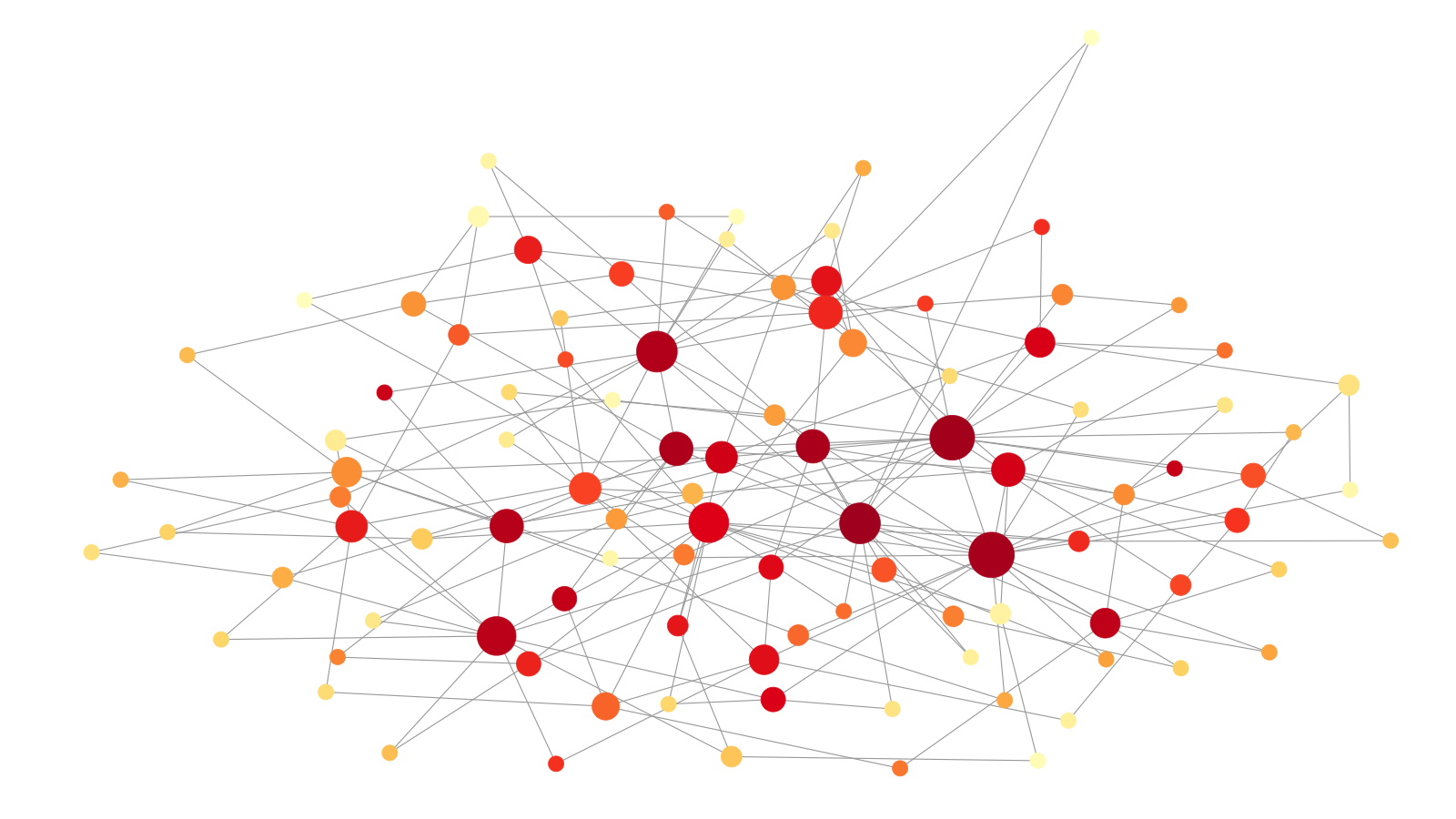
  #plot the new graph
  plot(gt,layout=layout.new,
       vertex.label="",vertex.size=1+2*log(degree(gt)),
       vertex.frame.color=V(A)$color,edge.width=1.5,
       asp=9/16,margin=-0.15)
  #use the new layout in the next round
  layout.old <- layout.new
}
dev.off()

Once you created the png image files of the network for each time step, then you can create an animation using “ffmpeg” application. If you already installed ‘brew’ in your computer, then you can easily install the “ffmpeg” with very short code like this in your terminal:

$ brew install ffmpeg

Then, you can create an network animation with the following code in your terminal:

ffmpeg -r 10 -i example%03d.png -b:v 20M output.mp4