Why is PISA Difficult to Analyze
By Byoung-gyu Gong

1. What is ILSA and PISA
International large-scale assessment (ILSA) is conducted regularly by international organizations to measure and compare many different countries’ educational performance and status. The Programme for International Student Assessment (PISA) by OECD is the most well-known ILSA testing member and non-member partner country’s 15-year-old students every two years. It measures students’ reading, math, and science using a computer-based instrument. It also surveys to collect more detailed background information of each student, teacher, and school. The PISA 2006 collected this massive size of data from 398,750 students. Thus, it can be said that the PISA is the most comprehensive large-sized international student assessment data set available now.
2. Why is it difficult to analyze PISA data
Despite the insightful knowledge we can gain from this large international students’ data set, PISA is not easily accessible to most of the researchers to analyze it. That is not because the data access is limited but because it is complexly structured, requesting sophisticated data pre-processing. Even Jerrim, Lopez-Agudo, Marcenaro-Gutierrez, and Shure (2017) said, “in spite of their acquired relevance, there are few studies which really account for the complex survey and test designs that they present and follow the technical procedures suggested by their developers” (p.1). I will illustrate what caution is needed to analyze the data set and provides R solution in this post using a data set of PISA 2006.
2.1. Two-staged sampling
The sampling design of the PISA is the reason why the analysis procedure is so complicated. The PISA does not use random sampling and instead follows two-staged sampling: sample schools and then sample students in the participating schools. It makes the sampling errors of population estimates increase. It conflicts with most computer software designed to assume random sampling for statistical analysis and requests more sophisticated analysis procedures. Once the assumption of random sampling is violated, the student data can depend on each other because they may share common school characteristics.
To avoid such bias, PISA made some complementary measures.
Once you look at the data table imported from the PISA 2006, you would see some strange variable names such as PV1-5 for each reading, math, and science domains. Also, there are some variables having names like W_FSTR1-80. If you just naively wanted to calculate students’ mean or correlation coefficient with a fixed point score, you would be embarrassed to find these unknown variables.
# Use the following packages for the analysis
library(intsvy)
library(dplyr)
library(ggplot2)head(pisa2006,1)## X CNT SCHOOLID STIDSTD PV1MATH PV2MATH PV3MATH PV4MATH PV5MATH PV1READ
## 1 1 ARG 1 1 305.1799 305.9589 264.6752 320.7587 301.2852 357.0519
## PV2READ PV3READ PV4READ PV5READ PV1SCIE PV2SCIE PV3SCIE PV4SCIE
## 1 312.1348 281.6554 316.9474 316.1453 395.3131 411.1652 445.6667 351.4869
## PV5SCIE PV1INTR PV2INTR PV3INTR PV4INTR PV5INTR PV1SUPP PV2SUPP
## 1 356.1492 539.9939 480.1177 497.9912 370.1956 506.0343 339.0228 395.3084
## PV3SUPP PV4SUPP PV5SUPP PV1EPS PV2EPS PV3EPS PV4EPS PV5EPS
## 1 412.5387 313.7517 322.9412 393.4482 384.1234 354.2843 430.7471 417.6925
## PV1ISI PV2ISI PV3ISI PV4ISI PV5ISI PV1USE PV2USE PV3USE
## 1 334.7023 304.8632 323.5126 399.9755 386.9209 401.8404 383.191 385.0559
## PV4USE PV5USE W_FSTUWT W_FSTR1 W_FSTR2 W_FSTR3 W_FSTR4 W_FSTR5 W_FSTR6
## 1 436.342 469.911 98.8278 52.1041 139.9112 52.1041 139.9112 52.1041 139.9112
## W_FSTR7 W_FSTR8 W_FSTR9 W_FSTR10 W_FSTR11 W_FSTR12 W_FSTR13 W_FSTR14 W_FSTR15
## 1 52.1041 52.1041 52.1041 52.1041 139.9112 139.9112 52.1041 139.9112 139.9112
## W_FSTR16 W_FSTR17 W_FSTR18 W_FSTR19 W_FSTR20 W_FSTR21 W_FSTR22 W_FSTR23
## 1 52.1041 52.1041 139.9112 139.9112 139.9112 52.1041 139.9112 52.1041
## W_FSTR24 W_FSTR25 W_FSTR26 W_FSTR27 W_FSTR28 W_FSTR29 W_FSTR30 W_FSTR31
## 1 139.9112 52.1041 139.9112 52.1041 52.1041 52.1041 52.1041 139.9112
## W_FSTR32 W_FSTR33 W_FSTR34 W_FSTR35 W_FSTR36 W_FSTR37 W_FSTR38 W_FSTR39
## 1 139.9112 52.1041 139.9112 139.9112 52.1041 52.1041 139.9112 139.9112
## W_FSTR40 W_FSTR41 W_FSTR42 W_FSTR43 W_FSTR44 W_FSTR45 W_FSTR46 W_FSTR47
## 1 139.9112 52.1041 139.9112 52.1041 139.9112 52.1041 139.9112 52.1041
## W_FSTR48 W_FSTR49 W_FSTR50 W_FSTR51 W_FSTR52 W_FSTR53 W_FSTR54 W_FSTR55
## 1 52.1041 52.1041 52.1041 139.9112 139.9112 52.1041 139.9112 139.9112
## W_FSTR56 W_FSTR57 W_FSTR58 W_FSTR59 W_FSTR60 W_FSTR61 W_FSTR62 W_FSTR63
## 1 52.1041 52.1041 139.9112 139.9112 139.9112 52.1041 139.9112 52.1041
## W_FSTR64 W_FSTR65 W_FSTR66 W_FSTR67 W_FSTR68 W_FSTR69 W_FSTR70 W_FSTR71
## 1 139.9112 52.1041 139.9112 52.1041 52.1041 52.1041 52.1041 139.9112
## W_FSTR72 W_FSTR73 W_FSTR74 W_FSTR75 W_FSTR76 W_FSTR77 W_FSTR78 W_FSTR79
## 1 139.9112 52.1041 139.9112 139.9112 52.1041 52.1041 139.9112 139.9112
## W_FSTR80 ESCS
## 1 139.9112 -2.0048Then, what are these variables in the PISA table?
2.2. Sampling Weight
To make each sampled student from each school represent each country’s entire population, we need to give a weight to each student variables. The random sample secures each sampled student’s equal probability, but two-stage sampling needs to adjust the probability with a complicated calculation of the weight. Weight is an inverse of probability to be selected as a sample. For instance, we selected ten students out of 100 students, then the probability to be selected is 0.1, and the weight is 10.
In PISA, each school’s probability to be selected is proportional to its size, which is called PPS sampling method. The schools with larger sizes have a higher probability of selection, but the larger schools have a proportionally less within-school probability of selection. The sum of students’ weight for each country is the total number of the students’ population assumed for the study.
There are two options to apply students’ weight for the PISA analysis, applying final weight(W_FSTUWT), and replicated weight(F_FSTR1-80), but in this post, I do not tackle the replicated weight because it is more related to the estimation of standard error, but not have an impact to the mean, correlation, and regression coefficent estimate.
Let me show you an example here with R code. W_FSTUWT is the final students’ weight. You can see that students in the same school have approximately the same school weights with a little variation. School number 00001 has weights around 98, and 00002 has it at about 89.
# Select Argentina students' weight information.
WEIGHT<-pisa2006 %>% select(CNT, SCHOOLID, W_FSTUWT) %>% filter(CNT=="ARG")
# Create a dataframe that can compare Argentina students in three different schools
A<-WEIGHT %>% filter(SCHOOLID=="1") %>% slice(1:3)
B<-WEIGHT %>% filter(SCHOOLID=="2") %>% slice(1:3)
C<-WEIGHT %>% filter(SCHOOLID=="3") %>% slice(1:3)
rbind(A,B,C)
## CNT SCHOOLID W_FSTUWT
## 1 ARG 1 98.8278
## 2 ARG 1 91.7075
## 3 ARG 1 98.8278
## 4 ARG 2 89.3573
## 5 ARG 2 89.6970
## 6 ARG 2 89.6970
## 7 ARG 3 112.7806
## 8 ARG 3 117.0837
## 9 ARG 3 117.0837The summation of the students’ weight is equal to the population total population of 15-years-old students in Argentina. It is 523,047.
WEIGHT %>% filter(CNT=="ARG") %>% group_by(CNT) %>% summarize(sum=sum(W_FSTUWT))## `summarise()` ungrouping output (override with `.groups` argument)## # A tibble: 1 x 2
## CNT sum
## <chr> <dbl>
## 1 ARG 523048.
Also, we can compare the difference in variable means between raw scores and weighted scores. Comparing with the graph ‘B’ with the graph ‘A,’ we can recognize that the graph ‘B’ is more slightly deviated from the regression line, although the difference is negligible for most countries. Some of the countries in specific variables, the bias to the estimate can be significantly large so we should apply the final student weight for the analysis all the time.
# Create weighted mean score (W_MEAN) and non-weighted means score of PV1SCIE (science score)
# Calculate national mean
PV1SCIE<-pisa2006 %>% select(CNT, PV1SCIE, W_FSTUWT) %>% group_by(CNT) %>%  mutate(W_MEAN=weighted.mean(PV1SCIE,W_FSTUWT, na.rm=TRUE), MEAN=mean(PV1SCIE, na.rm=TRUE)) %>% ungroup() %>% select(CNT, W_MEAN, MEAN) %>% unique()

# Create a scatter plot to compare the discrepancy between
library(ggplot2)
library(ggpubr)
# Create a scatter plot with raw score means (unweighted mean)
Non_weight<-ggplot(PV1SCIE, aes(x=MEAN, y=MEAN)) + geom_point() + geom_text(data=PV1SCIE, aes(label=CNT), position=position_jitter(width=0.1,height=0.1), size=3) + geom_smooth(method=lm, se=TRUE)+stat_cor(method = "pearson")
# Create a scatter plot with unweighted mean and weighted mean
Weight_non_weight<-ggplot(PV1SCIE, aes(x=MEAN, y=W_MEAN)) + geom_point() + geom_text(data=PV1SCIE, aes(label=CNT), position=position_jitter(width=0.1,height=0.1), size=3) + geom_smooth(method=lm, se=TRUE)+stat_cor(method = "pearson")
# Compore these two
ggarrange(Non_weight, Weight_non_weight,
          labels = c("A", "B"),
          ncol = 2, nrow = 1)
## `geom_smooth()` using formula 'y ~ x'
## `geom_smooth()` using formula 'y ~ x'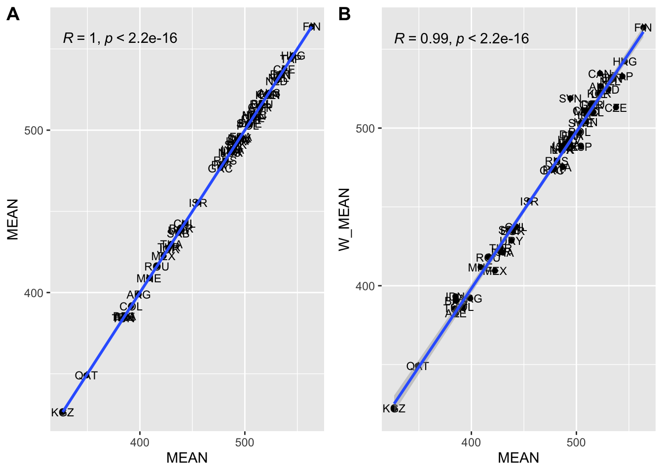
2.3. Plausible Value(PV)
PV is called plausible value, and each domain has five PVs. For instance, math has PV1MATH - PV5MATH, and science has PV1SCIE - PV5SCIE. The PVs are introduced here to adjust measurement error that can be caused by - the concept to be measured is not clear, - students physical and psychological condition affected at the moment of testing, and - the testing environment on a day of testing. Thus, if we have five different plausible values distributed in a certain range of raw scores, we can avoid point estimate of the students’ competency, which has a high risk of measurement error as mentioned above. It means that we interpret students’ competency as a probability distribution among the plausible values, not as a fixed point. In addition to this rational, the PV was adopted in a practical and efficient standpoint. In PISA tests, students do not take all the test items as it is time-consuming, and each student takes different sets of tests, while the test items missing in each student are treated as a missing value. It creates five different sets of literally plausible score values of the students.
I created two columns of mean data to compare weighted PV means and weighted means of each country. However, as we can see from the below table, there is no significant difference between the weighted PV mean and just the weighted mean with the final weight. The OECD also admitted that PV value does not bring significant impact to reduce bias in the estimate (OECD, 2009)
# Create a dataframe with weighted PV means (weighted by final weight)
PVSCIE<-pisa.mean.pv(pvlabel="SCIE", by="CNT", data=pisa2006)
# Create a dataframe with weighted means (weighted by final weight)
SCIE<-pisa2006 %>% group_by(CNT) %>% summarise(Mean=(weighted.mean(PV4SCIE,W_FSTUWT, na.rm=TRUE))) %>% mutate(Mean=round(Mean, 2))
## `summarise()` ungrouping output (override with `.groups` argument)Merge<-left_join(PVSCIE, SCIE, by="CNT") %>% select(CNT, Freq, Mean.x, Mean.y) %>% rename(PVmean="Mean.x", Rawmean="Mean.y")
head(Merge,15)## CNT Freq PVmean Rawmean
## 1 ARG 4339 391.24 391.33
## 2 AUS 14170 526.88 526.90
## 3 AUT 4927 510.84 510.95
## 4 AZE 5184 382.33 381.78
## 5 BEL 8857 510.36 510.62
## 6 BGR 4498 434.08 433.27
## 7 BRA 9295 390.33 389.43
## 8 CAN 22646 534.47 534.28
## 9 CHE 12192 511.52 511.71
## 10 CHL 5233 438.18 438.26
## 11 COL 4478 388.04 388.60
## 12 CZE 5932 512.86 512.69
## 13 DEU 4891 515.65 516.32
## 14 DNK 4532 495.89 495.05
## 15 ESP 19604 488.42 487.51
3. Conclusion
As we examined so far, the students’ final weight is a significant factor to reduce bias in estimation. Although PV value has less impact to the estimation and OECD also admit it, but still it should be best to follow the PISA instruction.
In this post, I only explored the estimates at each country level. However, it is very different for the case of cross-national analysis, setting each country as a unit of analysis. For instance, the weight that should be applied to each student should be adjusted. PISA also provides instruction on how to adjust the weight though there is still controversy over it. I will post this topic later on.
References
Jerrim, J., Lopez-Agudo, L. A., Marcenaro-Gutierrez, O. D., & Shure, N. (2017, June). To weight or not to weight?: the case of PISA data. In Proceedings of the XXVI Meeting of the Economics of Education Association, Murcia, Spain (pp. 29-30).
OECD (2009). PISA 2006 Technical Report. OECD Publishing.